Another important and useful family of distributions in statistics is the family of F-distributions. Each member of the F-distribution family is specified by a pair of parameters called degrees of freedom and denoted and Figure 11.7 "Many " shows several F-distributions for different pairs of degrees of freedom. An random variableA random variable following an F-distribution. is a random variable that assumes only positive values and follows an F-distribution.
Figure 11.7 Many F-Distributions
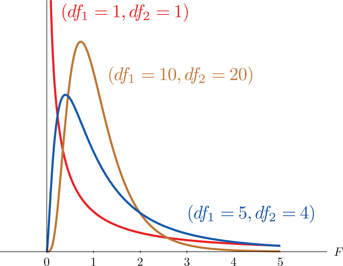
The parameter is often referred to as the numerator degrees of freedom and the parameter as the denominator degrees of freedom. It is important to keep in mind that they are not interchangeable. For example, the F-distribution with degrees of freedom and is a different distribution from the F-distribution with degrees of freedom and
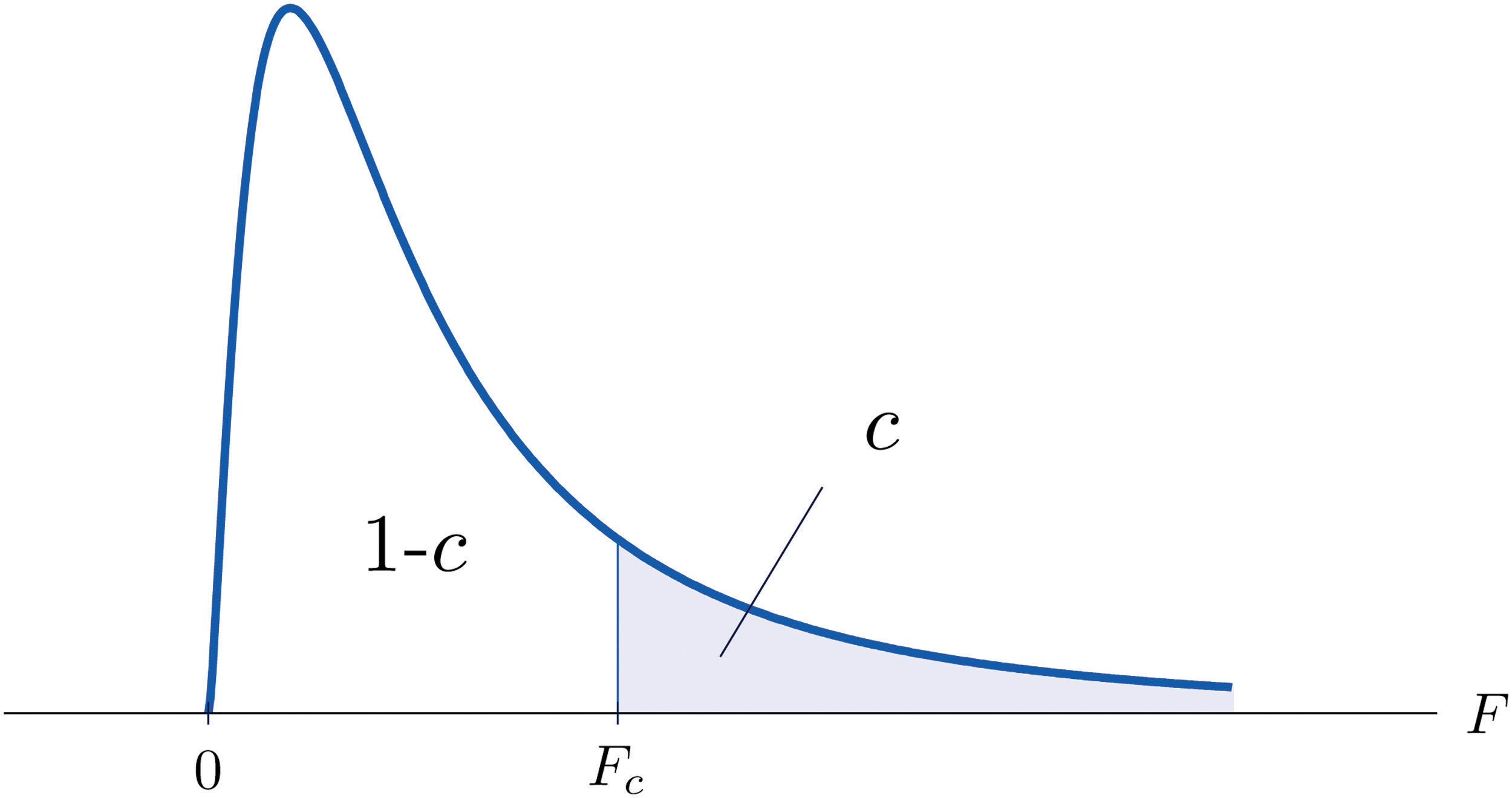
The value of the F random variable F with degrees of freedom and that cuts off a right tail of area c is denoted Fc and is called a critical value. See Figure 11.8.
Figure 11.8 Fc Illustrated
Tables containing the values of Fc are given in Chapter 11 "Chi-Square Tests and ". Each of the tables is for a fixed collection of values of c, either 0.900, 0.950, 0.975, 0.990, and 0.995 (yielding what are called “lower” critical values), or 0.005, 0.010, 0.025, 0.050, and 0.100 (yielding what are called “upper” critical values). In each table critical values are given for various pairs We illustrate the use of the tables with several examples.
Suppose F is an F random variable with degrees of freedom and Use the tables to find
Solution:
The column headings of all the tables contain Look for the table for which 0.10 is one of the entries on the extreme left (a table of upper critical values) and that has a row heading in the left margin of the table. A portion of the relevant table is provided. The entry in the intersection of the column with heading and the row with the headings 0.10 and , which is shaded in the table provided, is the answer,
| F Tail Area | 1 | 2 | 5 | |||
|---|---|---|---|---|---|---|
| ⋮ | ⋮ | ⋮ | ⋮ | ⋮ | ⋮ | ⋮ |
| 0.005 | 4 | 22.5 | ||||
| 0.01 | 4 | 15.5 | ||||
| 0.025 | 4 | 9.36 | ||||
| 0.05 | 4 | 6.26 | ||||
| 0.10 | 4 | |||||
| ⋮ | ⋮ | ⋮ | ⋮ | ⋮ | ⋮ | ⋮ |
Look for the table for which 0.95 is one of the entries on the extreme left (a table of lower critical values) and that has a row heading in the left margin of the table. A portion of the relevant table is provided. The entry in the intersection of the column with heading and the row with the headings 0.95 and , which is shaded in the table provided, is the answer,
| F Tail Area | 1 | 2 | 5 | |||
|---|---|---|---|---|---|---|
| ⋮ | ⋮ | ⋮ | ⋮ | ⋮ | ⋮ | ⋮ |
| 0.90 | 4 | 0.28 | ||||
| 0.95 | 4 | |||||
| 0.975 | 4 | 0.14 | ||||
| 0.99 | 4 | 0.09 | ||||
| 0.995 | 4 | 0.06 | ||||
| ⋮ | ⋮ | ⋮ | ⋮ | ⋮ | ⋮ | ⋮ |
Suppose is an F random variable with degrees of freedom and Let Use the tables to find
Solution:
The column headings of all the tables contain Look for the table for which is one of the entries on the extreme left (a table of upper critical values) and that has a row heading in the left margin of the table. A portion of the relevant table is provided. The shaded entry, in the intersection of the column with heading and the row with the headings 0.05 and is the answer,
| F Tail Area | 1 | 2 | ||
|---|---|---|---|---|
| ⋮ | ⋮ | ⋮ | ⋮ | ⋮ |
| 0.005 | 20 | 6.99 | ||
| 0.01 | 20 | 5.85 | ||
| 0.025 | 20 | 4.46 | ||
| 0.05 | 20 | |||
| 0.10 | 20 | 2.59 | ||
| ⋮ | ⋮ | ⋮ | ⋮ | ⋮ |
Look for the table for which is one of the entries on the extreme left (a table of upper critical values) and that has a row heading in the left margin of the table. A portion of the relevant table is provided. The shaded entry, in the intersection of the column with heading and the row with the headings 0.025 and is the answer,
| F Tail Area | 1 | 2 | ||
|---|---|---|---|---|
| ⋮ | ⋮ | ⋮ | ⋮ | ⋮ |
| 0.005 | 20 | 6.99 | ||
| 0.01 | 20 | 5.85 | ||
| 0.025 | 20 | |||
| 0.05 | 20 | 3.49 | ||
| 0.10 | 20 | 2.59 | ||
| ⋮ | ⋮ | ⋮ | ⋮ | ⋮ |
Look for the table for which is one of the entries on the extreme left (a table of lower critical values) and that has a row heading in the left margin of the table. A portion of the relevant table is provided. The shaded entry, in the intersection of the column with heading and the row with the headings 0.95 and is the answer,
| F Tail Area | 1 | 2 | ||
|---|---|---|---|---|
| ⋮ | ⋮ | ⋮ | ⋮ | ⋮ |
| 0.90 | 20 | 0.11 | ||
| 0.95 | 20 | |||
| 0.975 | 20 | 0.03 | ||
| 0.99 | 20 | 0.01 | ||
| 0.995 | 20 | 0.01 | ||
| ⋮ | ⋮ | ⋮ | ⋮ | ⋮ |
Look for the table for which is one of the entries on the extreme left (a table of lower critical values) and that has a row heading in the left margin of the table. A portion of the relevant table is provided. The shaded entry, in the intersection of the column with heading and the row with the headings 0.975 and is the answer,
| F Tail Area | 1 | 2 | ||
|---|---|---|---|---|
| ⋮ | ⋮ | ⋮ | ⋮ | ⋮ |
| 0.90 | 20 | 0.11 | ||
| 0.95 | 20 | 0.05 | ||
| 0.975 | 20 | |||
| 0.99 | 20 | 0.01 | ||
| 0.995 | 20 | 0.01 | ||
| ⋮ | ⋮ | ⋮ | ⋮ | ⋮ |
A fact that sometimes allows us to find a critical value from a table that we could not read otherwise is:
If denotes the value of the F-distribution with degrees of freedom and that cuts off a right tail of area u, then
Use the tables to find
Solution:
There is no table with , but there is one with Thus we use the fact that
Using the relevant table we find that , hence
There is no table with , but there is one with Thus we use the fact that
Using the relevant table we find that , hence
A test based on an F statistic to check whether two population variances are equal.In Chapter 9 "Two-Sample Problems" we saw how to test hypotheses about the difference between two population means and In some practical situations the difference between the population standard deviations and is also of interest. Standard deviation measures the variability of a random variable. For example, if the random variable measures the size of a machined part in a manufacturing process, the size of standard deviation is one indicator of product quality. A smaller standard deviation among items produced in the manufacturing process is desirable since it indicates consistency in product quality.
For theoretical reasons it is easier to compare the squares of the population standard deviations, the population variances and This is not a problem, since precisely when , precisely when , and precisely when
The null hypothesis always has the form The three forms of the alternative hypothesis, with the terminology for each case, are:
| Form of Ha | Terminology |
|---|---|
| Right-tailed | |
| Left-tailed | |
| Two-tailed |
Just as when we test hypotheses concerning two population means, we take a random sample from each population, of sizes n1 and n2, and compute the sample standard deviations s1 and s2. In this context the samples are always independent. The populations themselves must be normally distributed.
If the two populations are normally distributed and if is true then under independent sampling F approximately follows an F-distribution with degrees of freedom and
A test based on the test statistic is called an F-test.
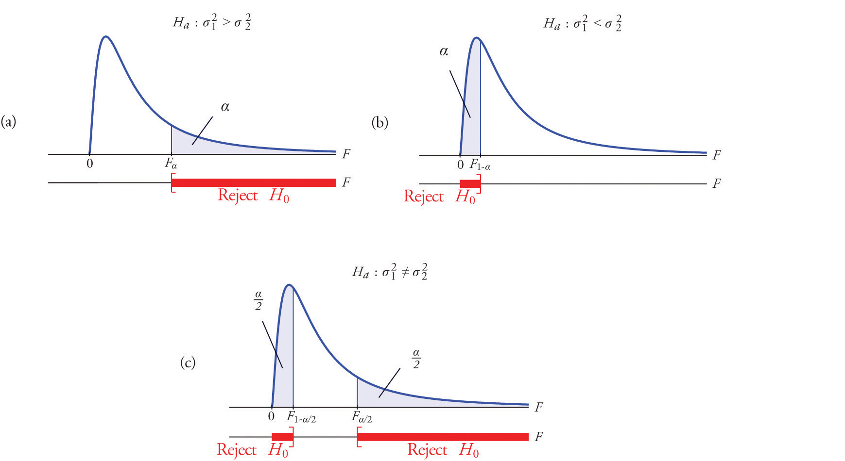
A most important point is that while the rejection region for a right-tailed test is exactly as in every other situation that we have encountered, because of the asymmetry in the F-distribution the critical value for a left-tailed test and the lower critical value for a two-tailed test have the special forms shown in the following table:
| Terminology | Alternative Hypothesis | Rejection Region |
|---|---|---|
| Right-tailed | ||
| Left-tailed | ||
| Two-tailed | or |
Figure 11.9 "Rejection Regions: (a) Right-Tailed; (b) Left-Tailed; (c) Two-Tailed" illustrates these rejection regions.
Figure 11.9 Rejection Regions: (a) Right-Tailed; (b) Left-Tailed; (c) Two-Tailed
The test is performed using the usual five-step procedure described at the end of Section 8.1 "The Elements of Hypothesis Testing" in Chapter 8 "Testing Hypotheses".
One of the quality measures of blood glucose meter strips is the consistency of the test results on the same sample of blood. The consistency is measured by the variance of the readings in repeated testing. Suppose two types of strips, A and B, are compared for their respective consistencies. We arbitrarily label the population of Type A strips Population 1 and the population of Type B strips Population 2. Suppose 15 Type A strips were tested with blood drops from a well-shaken vial and 20 Type B strips were tested with the blood from the same vial. The results are summarized in Table 11.16 "Two Types of Test Strips". Assume the glucose readings using Type A strips follow a normal distribution with variance and those using Type B strips follow a normal distribution with variance with Test, at the 10% level of significance, whether the data provide sufficient evidence to conclude that the consistencies of the two types of strips are different.
Table 11.16 Two Types of Test Strips
| Strip Type | Sample Size | Sample Variance |
|---|---|---|
| A | ||
| B |
Solution:
Step 1. The test of hypotheses is
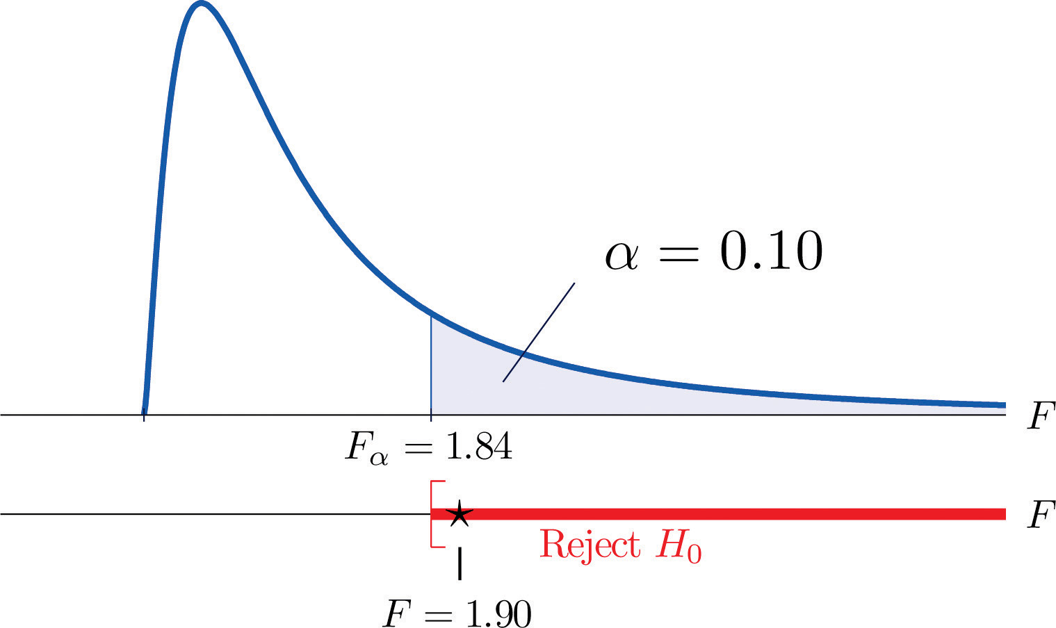
Figure 11.10 Rejection Region and Test Statistic for Note 11.27 "Example 6"
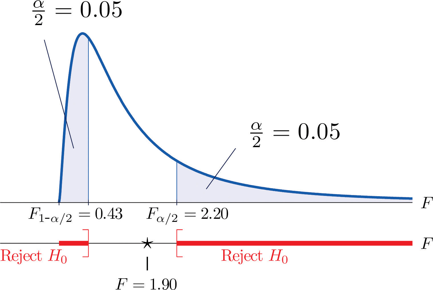
Step 4. The value of the test statistic is
In the context of Note 11.27 "Example 6", suppose Type A test strips are the current market leader and Type B test strips are a newly improved version of Type A. Test, at the 10% level of significance, whether the data given in Table 11.16 "Two Types of Test Strips" provide sufficient evidence to conclude that Type B test strips have better consistency (lower variance) than Type A test strips.
Solution:
Step 1. The test of hypotheses is now
Step 3. The value of the test statistic is
Figure 11.11 Rejection Region and Test Statistic for Note 11.28 "Example 7"
Find F0.01 for each of the following degrees of freedom.
Find F0.05 for each of the following degrees of freedom.
Find F0.95 for each of the following degrees of freedom.
Find F0.90 for each of the following degrees of freedom.
For , and , find
For , , and , find
For each of the two samples
find
For each of the two samples
find
Two random samples taken from two normal populations yielded the following information:
| Sample | Sample Size | Sample Variance |
|---|---|---|
| 1 | ||
| 2 |
Two random samples taken from two normal populations yielded the following information:
| Sample | Sample Size | Sample Variance |
|---|---|---|
| 1 | ||
| 2 |
Two random samples taken from two normal populations yielded the following information:
| Sample | Sample Size | Sample Variance |
|---|---|---|
| 1 | ||
| 2 |
Two random samples taken from two normal populations yielded the following information:
| Sample | Sample Size | Sample Variance |
|---|---|---|
| 1 | ||
| 2 |
Two random samples taken from two normal populations yielded the following information:
| Sample | Sample Size | Sample Variance |
|---|---|---|
| 1 | ||
| 2 |
Two random samples taken from two normal populations yielded the following information:
| Sample | Sample Size | Sample Variance |
|---|---|---|
| 1 | ||
| 2 |
Japanese sturgeon is a subspecies of the sturgeon family indigenous to Japan and the Northwest Pacific. In a particular fish hatchery newly hatched baby Japanese sturgeon are kept in tanks for several weeks before being transferred to larger ponds. Dissolved oxygen in tank water is very tightly monitored by an electronic system and rigorously maintained at a target level of 6.5 milligrams per liter (mg/l). The fish hatchery looks to upgrade their water monitoring systems for tighter control of dissolved oxygen. A new system is evaluated against the old one currently being used in terms of the variance in measured dissolved oxygen. Thirty-one water samples from a tank operated with the new system were collected and 16 water samples from a tank operated with the old system were collected, all during the course of a day. The samples yield the following information:
Test, at the 10% level of significance, whether the data provide sufficient evidence to conclude that the new system will provide a tighter control of dissolved oxygen in the tanks.
The risk of investing in a stock is measured by the volatility, or the variance, in changes in the price of that stock. Mutual funds are baskets of stocks and offer generally lower risk to investors. Different mutual funds have different focuses and offer different levels of risk. Hippolyta is deciding between two mutual funds, A and B, with similar expected returns. To make a final decision, she examined the annual returns of the two funds during the last ten years and obtained the following information:
Test, at the 5% level of significance, whether the data provide sufficient evidence to conclude that the two mutual funds offer different levels of risk.
It is commonly acknowledged that grading of the writing part of a college entrance examination is subject to inconsistency. Every year a large number of potential graders are put through a rigorous training program before being given grading assignments. In order to gauge whether such a training program really enhances consistency in grading, a statistician conducted an experiment in which a reference essay was given to 61 trained graders and 31 untrained graders. Information on the scores given by these graders is summarized below:
Test, at the 5% level of significance, whether the data provide sufficient evidence to conclude that the training program enhances the consistency in essay grading.
A common problem encountered by many classical music radio stations is that their listeners belong to an increasingly narrow band of ages in the population. The new general manager of a classical music radio station believed that a new playlist offered by a professional programming agency would attract listeners from a wider range of ages. The new list was used for a year. Two random samples were taken before and after the new playlist was adopted. Information on the ages of the listeners in the sample are summarized below:
Test, at the 10% level of significance, whether the data provide sufficient evidence to conclude that the new playlist has expanded the range of listener ages.
A laptop computer maker uses battery packs supplied by two companies, A and B. While both brands have the same average battery life between charges (LBC), the computer maker seems to receive more complaints about shorter LBC than expected for battery packs supplied by company B. The computer maker suspects that this could be caused by higher variance in LBC for Brand B. To check that, ten new battery packs from each brand are selected, installed on the same models of laptops, and the laptops are allowed to run until the battery packs are completely discharged. The following are the observed LBCs in hours.
Test, at the 5% level of significance, whether the data provide sufficient evidence to conclude that the LBCs of Brand B have a larger variance that those of Brand A.
A manufacturer of a blood-pressure measuring device for home use claims that its device is more consistent than that produced by a leading competitor. During a visit to a medical store a potential buyer tried both devices on himself repeatedly during a short period of time. The following are readings of systolic pressure.
Large Data Sets 1A and 1B record SAT scores for 419 male and 581 female students. Test, at the 1% level of significance, whether the data provide sufficient evidence to conclude that the variances of scores of male and female students differ.
https://www.gone.2012books.lardbucket.org/sites/all/files/data1A.xls
https://www.gone.2012books.lardbucket.org/sites/all/files/data1B.xls
Large Data Sets 7, 7A, and 7B record the survival times of 140 laboratory mice with thymic leukemia. Test, at the 10% level of significance, whether the data provide sufficient evidence to conclude that the variances of survival times of male mice and female mice differ.
https://www.gone.2012books.lardbucket.org/sites/all/files/data7.xls
https://www.gone.2012books.lardbucket.org/sites/all/files/data7A.xls
https://www.gone.2012books.lardbucket.org/sites/all/files/data7B.xls
Sample 1:
Sample 2:
F = 0.3793, , reject H0
F = 0.5499, , reject H0
F = 0.0971, , reject H0
F = 0.893131. and Rejection Region: Decision: Fail to reject H0 of equal variances.


